The Improbability Principle

This is part one of my takeaways I’ve learnt from the book The Improbability Principle by David J. Hand. It explores the reasons behind why very rare things do occur. I’ve selected quotes and explanations from the book, paraphrased them and added my own findings to the mix. Enjoy!

Introduction

• As humans, we are naturally curious and tend to be on the lookout for coincidences and patterns we find in everyday life.
• Of course, there are many interesting coincidences.
  • From Carl Jung’s Synchronity: Writer Wilhelm von Scholz tells the story of a mother who photographed her son in 1914 and sent the film to be developed in Strassburg. However war broke out and she could not retrieve it. Two years later, in Frankfurt, she bought a roll of film to photograph her daughter – when she developed the film she found another picture overlaid on the film – it was the photograph of her son in 1914! The old film must have been accidentally recirculated to be sold with the new films. ¹
  • Or Major Summerford, who was struck by lightning 3 times over the course of his life ² – and lightning struck his gravestone as well. The probability of being struck by lightning outdoors is 1 in 750,000.

But perhaps coincidences are the reason behind our reality as we know it –

• (Darwin’s Theory of Evolution) Tiny random changes in DNA caused us to evolve from water-dwelling creatures into humans.
• (Maxwell’s Equations) Why is the speed of light exactly 299,792,458 m/s?

Borel’s Law

Events With A Sufficiently Small Probability Never Occur

Émile Borel, a French mathematician born in 1871, was a trailblazer for mathematical methods regarding probability.

Borel’s Law is in regards to the Infinite Monkey Theorem – a monkey who randomly presses letters on a typewriter, given an infinite amount of time would be able to reproduce any works of literature exactly, like the complete works of Shakespeare.

However, without an infinite amount of time, this event would could not be rationally demonstrated, and could be considered actually impossible. This law relates to probabilities so small that it would be irrational to witness it ever happen within the span of human existence.³

But this threshold still applies to the less far-fetched. Borel’s writes, “For every Parisian who circulates for one day, the probability of being killed in the course of the day in a traffic accident is about one-millionth. If, in order to avoid this slight risk, a man renounced all external activity and cloistered himself in his house, or imposed such confinement on his wife or his son, he would be considered mad.”⁴

Borel’s Law takes a practicality stance when it comes to probabilities – treat very tiny probabilities as if they were zero. He also gives a scale of negligence and names for each extent of improbability.

1. Negligible on the human scale: 1 in 650,000. One example of this is being dealt a royal flush in poker.
2. Negligible on the terrestrial scale: 1 in 10^15. One example is dividing the earth into square feet (earth’s surface area is 5.5 * 10^15 sqf). Suppose you and I choose one square foot at random, the probability of us choosing the same square would be on the terrestrial scale.
3. Negligible on the cosmic scale: 1 in 10^50. Earth has 10^50 atoms, so this probability is the same as two people randomly choosing the same atom on the Earth.
4. Negligible on the supercosmic scale: 1 in 10^1000,000,000. This is such a huge number; even greater than the number of subatomic particles in the universe. The book provides no examples for this.

But Borel’s Law…

Yes, but the Improbability Principle tells us that highly unlikely events keep occurring. We still see them from time to time. Now this creates a contradiction.

Things we get wrong as humans:

Humans are naturally curious and will look for patterns – however, sometimes, correlation does not mean causation.

1. “Hot hand” play. When players are on a winning streak, onlookers think that they are more likely to continue scoring higher than average, even though their performance is purely random. Numbers do repeat in sequences randomly – see point 6.

2. Superstitions such as walking under a ladder bringing bad luck. This could be due to a pot of paint dropped on you while walking underneath a ladder. A similar example would be the trivial rituals sports players undertake before starting a game. For example, a certain sock combination, a lucky hat, cutting fingernails at half-time.

   Once a superstition is established, they tend to strengthen on their own. This is due to confirmation bias – humans are not good at testing hypothesis easily as we only capitalise on evidence and events that support our theories.

3. Prophecies. Prophecies are not the same as predictions. Predictions are made from accumulated evidence and statistical methods of evaluation. Examples of predictions can be weather predictions based on wind speed, humidity, temperature, and season. But prophecies are based on uncertainties.

   Take Nostradamus’s prophecies, foretelling future natural disasters and wars, as an example. The reasons why some people believe his claims are legitimate are because of confirmation bias and the law of near-enough. I’ll cover on the latter cause, but for now, the name is self-explanatory – Prophecies are usually ambiguous and can be interpreted to be correct. Confirmation bias is at work here – his supporters only focus on/publish the prophecies he got right, leaving out the untrue prophecies, which actually outnumbered his correct prophecies.

   There are also self-fulfilling prophecies – a term coined by sociologist Robert K. Merton, for example, a student who believes he will fail an exam, will spend more time worrying than studying, which will affect his mental performance; he ends up failing the exam. ⁵

   Optimists tend to put themselves in positions with favourable outcomes and the opposite happens for pessimists. But perhaps optimists spent more time looking for improvements in outcomes than their negative counterparts, and were more likely to find it.

4. Conjunction Fallacy.

   Read the following question.

   John is male. Which is more likely?

   A: John is married with two children.

   B: John is married with two children, enjoys fishing and playing computer games.

   Many people answer B as they percieve the combinations of two independent events are more likely than one event, even though B is a duplicate of A and more, which means the probability of B should be less than A.

   People are shaped by their stereotypes and biases, as they most likely came up with an image of John, a male, doing hobbies that are more male-oriented.

5. Prosecutor’s Fallacy.

   There is a trial for a murder case – see the data below.

6. 

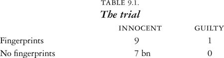
   A defendant is at trial, being accused of the murder because his fingerprints were found at the scene.

   The probability of his innocence is 0.9, as there are 9 fingerprints out of 10.

   The probability of his fingers being at the scene (yet still innocent) would be 9/(7bn + 9)≈ 1.286*10^-9.

   Now, the judge might focus too much on the second probability because it would be a 1 in 77,777,7779 chance – very suspicious.

   But the more important probability we should focus on is the 0.9 value – he is more likely to be innocent!

7. We are not good at generating random numbers. If were asked to imitate a random number generator from 1-10 we would avoid repeating the same number, trying to balance everything out. Humans are not used to repeated digits in random sequences. Apple had a ‘shuffle’ feature on their iPods, and in 2008 some people complained that the shuffle wasn’t ‘random enough’ ⁶, as they would hear songs from the same artist or album played consecutively. Although these sequences were expected from random list of songs, Apple had to tweak it so similar songs wouldn’t play together.

8. Hindsight bias – It is easy to see the signs leading to an event once know it has happened. Take the 9/11 tragedy for example, it is possible to see the events hinting the attack, but that is in retrospect. There are simply too many combinations to fit the pieces together, but knowing the outcome makes it much easier to come up with a explanation. In fact, we see many inverse examples – people making confident predictions that with hindsight turned out to be the opposite.

   1. “The horse is here to stay, but the automobile is only a novelty, a fad.” – President of Michigan Savings Bank, advising Henry Ford’s lawyer not to invest in the Ford Motor Company
   2. “There is no reason for any individual to have a computer in his home.” – Ken Olson, president of the Digital Equipment Corporation
   3. “There’s no chance that the iPhone is going to get any significant market share.” Steve Ballmer, 2007

Gambler’s fallacy

When tossing a coin repeatedly, in the event one side keeps getting tossed more than the other, many people expect the other side of the coin to have a higher chance of being tossed to ‘counterbalance‘ the disparity. However, this is not the case. What happens is that the later tosses should have roughly equal numbers of head and tails, and this equality dilutes the earlier disparity, given a large number of tosses. Keep in mind how this works – eventually when you toss the coin a very large number of times, you will get a perfect 50-50 split. This ties in with the Law of Large Numbers that I’ll come to in a moment.

A Clockwork Universe

Pierre Simon, a 17th-century mathematician wrote:

“An intelligence which, at a given instant, would know all the forces by which Nature is animated, and the respective situation of all the elements of which it is composed, if furthermore it were vast enough to submit all these data to analysis, would in the same formula encompass the motions of the largest bodies of the universe, and those of the most minute atom: nothing for it would be uncertain, and the future as well as the past would be present to its eyes.”

His view of nature is also known as as a clockwork universe – describing a deterministic universe, progressing forward, ticking along a pre-determined route. The only obstacle hindering the prediction of natural phenomena was simply ignorance – or undiscovered conditions or situations masking the situation. As science advances, this ignorance would be eroded, e.g. with the advent of microscopes.

However, over the 20th century, this ironic theory, or rather, ignorance eroded away. Quantum physics became a debated new topic, and it seemed that the universe was run by random chance and uncertainties. The term chaos comes into place here.

Edward Lorenz, the founder of chaos theory, summarised this: ”Chaos: when the present determines the future, but the approximate present does not approximately determine the future.” ⁷

We only have approximate knowledge about the present. The system of physics as we know it is an intrinsically unstable at its core – given the quantum properties of nature on an atomic scale. For example, trying to balance a pencil on its point. It will eventually fall, and the direction of how it falls is dependent on its minute differences in its position at the start. Also, think of cue balls on a snooker table – how they collide and rebound off each other is dependent on the angle of attack, speed, the surface of the table, and even the wear and tear on the stick and the cue ball. Minute differences in initial conditions will influence the outcome, making prediction impossible.

Then, we can never measure anything with perfect accuracy.

Chaos: Randomness vs Predictability

Keep in mind that randomness and predictability are mutually exclusive. Randomness refers to the unpredictable, flow of events, or a notion of free will. Outcomes can be assigned different probabilities but it will be impossible to determine the sequence of the outcomes exactly.

Predictability, however, is the opposite of randomness – for example, we can predict a sequence of numbers generated by a chaotic system, provided we have complete knowledge of the system and the starting value. Another word for this ‘chaotic system’, in computer science, is also called a pseudorandom number generator.

Law of Large Numbers

The average of a sequence of numbers randomly drawn from a given set of values is likely to get closer and closer to the average of that set.

Consider the set of 6 values {1, 2, 3, 4, 5, 6}. They have an average of 3.5.

Supposing we choose randomly pick a number from the set (we don’t take it out, so we can pick it more than once.) The more we randomly pick out each number, the closer the average of the picks get to 3.5. We could generate a number by throwing a 6-sided die.

If you only pick out a few numbers, the average of the values start to jump around, for from the value of 3.5 we’re looking for. But gradually, as more throws are made, the more the average settles down and converges towards 3.5. We learn the proper terminology in A-Level Statistics; that the average of the picks is E(X)/n, where E(X) is the expected value of the throws added together and n is the number of throws. (Given that the probabilities are spread across a discrete uniform distribution).

The Law of Large Numbers shows that it is important to have many participants in a clinical trial – a smaller number of participants allows for greater variability (from the mean performance of the drug), which may not be an accurate representation of how effective a drug is. A greater number of participants dilutes any variability and improves the accuracy of the trial.

Central Limit Theorem

Imagine choosing values at random from the set {1, 2, 3, 4, 5, 6}, where the selection is done by a fair 6-sided die. Five values are to be drawn and their average calculated. Another 5 values are drawn and another average is also calculated. These two averages are likely to be different. Once we repeat the calculation of the averages many times, we end up with a distribution of averages for a sample size of five (which you could plot on a graph.)

Well, we could have used different sample sizes instead of 5. But the central limit theorem describes the shape of distribution that we would achieve as larger and larger sample sizes are used. This is known as the normal distribution, which takes the shape of a bell.

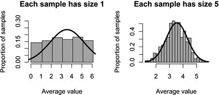
(Diagram taken from The Improbability Principle by David J. Hand)

End of Part 1

We’ve gone through limitations of the human mind when it comes to probabilities. I’ve set the stage by explaining the concept of chaos, large numbers, and how to obtain the normal distribution. This knowledge of the normal distribution may come in useful for part 2.

You can read part 2 here: